FlowSat generates 512 px satellite imagery from a caption and the
acquisition metadata that defines how the image was captured — where on
Earth, at what ground resolution, on what date, under how much cloud. Most
text-to-image models fold such metadata, when they use it at all, into a
single undifferentiated vector added to the timestep embedding. FlowSat
encodes each field on its own geometry and injects the result through a
zero-initialised graft on the pretrained modulation path, so metadata
influence is learned rather than imposed. On FMoW-RGB it reaches
FID 28.74 in 20 sampling steps, against 35.27 in 100 for the closest prior
work.
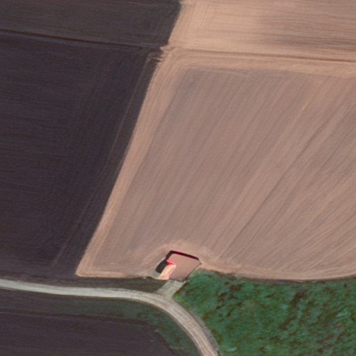
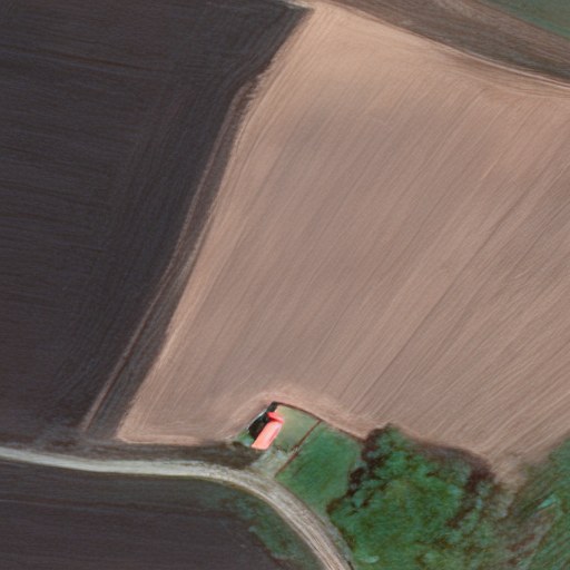
Metadata is the dial. One caption, one noise seed.
Only the acquisition month changes, left to right.
Interactive
Turn the dial yourself
Every image below was generated from the same caption
and the same noise seed. Only one metadata field changes. Drag a
slider to see what that field controls.
generate sweeps into static/sweeps/
MonthJuly
Comparison
Same prompt, different acquisition
Drag the divider. Both sides share a caption and a seed; only the metadata
differs.
static/compare/a.jpg + static/compare/b.jpg
⇆
JanuaryJuly
Method
How it works
Satellite imagery is defined as much by how it was
captured as by what it contains. Captions rarely state the season, the
sensor resolution or the atmosphere — yet those are exactly what a
user wants to control.
The seven fields
Conditioning is seven numbers, normalised to a common range. A caption
almost never states any of them.
Field
Encoded as
What it moves in the image
Longitude, latitude
Lifted onto the unit sphere, then expanded over many frequencies
Biome, building and field geometry, road pattern, materials
Month, day
Cyclically, so December sits next to January
Season — vegetation, snow, sun angle and shadow length
Year
On its own scale
Sensor generation, and how built-up the scene is
Ground sample distance
On its natural metres-per-pixel scale
How much ground one pixel covers: scale, and which objects resolve at all
Cloud cover
On its own scale
Haze, contrast, and outright occlusion
Encoding each field on the geometry it actually lives on is the point.
Coordinates are a position on a sphere, not two independent numbers, so
places either side of the dateline stay neighbours. Dates are a circle, so
December neighbours January. Ground resolution is a scalar spanning an
order of magnitude. Folding all seven into one flat vector throws that
structure away before the model sees it.
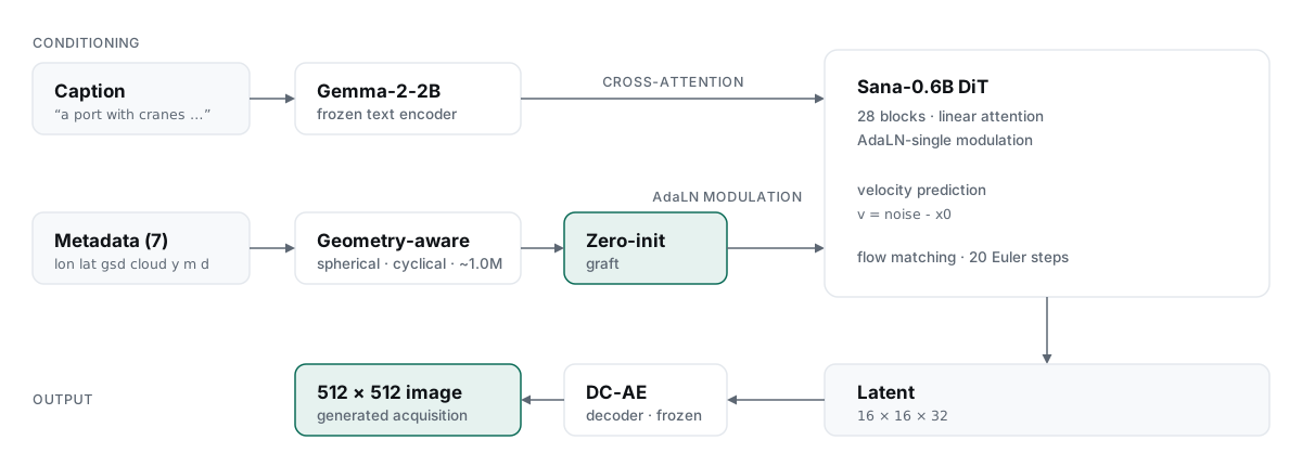
The resulting embedding does not get its own new pathway into the network.
It joins the modulation signal the pretrained backbone already uses, through
a projection initialised to exactly zero — so at step
0 the model is byte-identical to the text-to-image checkpoint it started
from, and every unit of metadata influence has to be earned by gradient
descent rather than imposed by construction.
Flow matching, not denoising
Training does not add noise in steps and learn to undo it. It draws a
straight path between a real latent and a sample of noise,
xt = (1−t)·x₀ + t·ε,
and learns the constant velocity along that path,
v = ε − x₀. Generation integrates the
velocity back from noise with an Euler solver. Because the path is straight,
few steps suffice — 20 rather than the 100 a denoising sampler needs.
The backbone is natively flow-matched, so time is used directly in [0, 1]
with no timestep rescaling.
Geometry-aware encoding
Sphere for coordinates, circle for dates, natural scale for resolution
and cloud — 1.04M parameters, an order of magnitude smaller than a
naive per-field MLP and measurably better.
Zero-initialised graft
Metadata joins the modulation the backbone already uses, through a
projection starting at zero. No new pathway, and no perturbation of the
pretrained prior at initialisation.
Flow matching
Velocity prediction along a straight path, on a backbone pretrained the
same way. Quality samples in 20 Euler steps rather than 100 denoising
steps.
Efficient backbone
Sana-0.6B, linear attention, and a DC-AE compressing 32× in each
direction — a whole 512 px frame is 256 latent tokens. Text
comes from a frozen Gemma-2-2B.
Results
FMoW-RGB at 512 px
Identical FID reference statistics and sample set across all models.
Model
FID ↓
CLIP ↑
Steps
DiffusionSat (ICLR 2024)
35.27
0.1720
100
GeoDiT-2Σ
32.11
—
—
FlowSat (ours, as submitted)
31.10
0.3016
20
FlowSat (ours, this release)
28.74
0.3019
20
Three-seed variance, as submitted:
FID 31.53 ± 0.32, CLIP 0.3018 ± 0.0007. The step-count advantage
derives from flow matching and the DC-AE/Sana backbone rather than from
metadata conditioning; the encoder's own contribution is isolated in the
ablation.
On the two FlowSat rows. The released
checkpoint and the released evaluation code give FID 28.74,
not the 31.10 printed in the paper. We report both rather than quietly
replacing one with the other. The gap is not the evaluation code: three
independent runs — this repository's
evaluate_fmow.py on its defaults, the same script on the
paper-submission text-encoder path, and the original unreleased script that
produced the submitted number — agree with each other to within
0.02 FID, all landing at 28.72–28.74 on the same
checkpoint, captions and protocol. We have not identified what differed in
the submitted run. The number moved in the favourable direction, and the
ranking against prior work is unchanged; the figure to reproduce from this
repository is 28.74.
Reproducing these numbers
One script measures all four reported metrics under the published
protocol — 10,000 FMoW test samples, 20 Euler steps, guidance 2.5,
seed 42. It writes the protocol it ran under alongside the results, so two
runs can be checked against each other before their numbers are compared.
On one A100 the run above takes
about 64 minutes and scores 9,999 of 10,000 — one FMoW test GeoTIFF
is unreadable and is dropped rather than substituted.
FID against sample count
FID is biased upward at small N, so a number measured at one sample count
cannot be compared with a number measured at another. Every row below comes
from the same generation pass, read at increasing counts:
N scored
FID ↓
CLIP ↑
5,007
35.93
0.3021
6,007
33.64
0.3017
7,007
31.93
0.3017
8,007
30.43
0.3019
9,007
29.42
0.3018
9,999
28.74
0.3019
CLIP is flat across the sweep;
FID is not. A run that stops early reports a worse FID than it earned, which
is the single most common reason a reproduction disagrees.
The same run reports the paired
reconstruction metrics, SSIM 0.1564 and
LPIPS 0.6574. Those score each image against the one real
acquisition its caption and metadata came from, so they measure
conditioning fidelity rather than image quality: two real FMoW
images of the same place reach only SSIM 0.214 / LPIPS 0.425 through the
same pipeline.
→Reproducing the evaluation — what each
metric measures here, and what has to match before two runs are comparable.
Samples
Controllability
What makes a model metadata-controllable
Metadata conditioning either works or quietly does nothing,
and the difference is rarely the architecture.
A generative model has to explain the variation in its training images,
and every conditioning signal competes to do that explaining. Text is
cheap: it arrives through a large pretrained encoder, cross-attended at
every block. Metadata is expensive: a small learned embedding through a
narrow injection path. So when a caption already states what a metadata
field encodes, that field is redundant during training — gradient
descent routes around it, the pathway starves, and at inference the field
looks inert. The model is behaving correctly; there was nothing left for
it to explain.
Controllability is inversely proportional to how much your
captions cover that field's own domain. The mechanism is
overlap, not richness: a 300-word caption about rooftop geometry
and pavement texture leaves latitude's variance untouched, while a
30-word "an arid Egyptian site in winter" destroys it.
The caption mixture we train on
Bucket
Share
Why
Rich VLM caption
40%
Image quality and text fidelity
Short template caption
30%
Keeps brief prompts in distribution
Empty caption
30%
The only regime where metadata must carry the load alone
The empty bucket is the one
people omit. Our earlier 70:20:10 split left only 10% caption-free samples
and produced visibly weaker metadata response than 40:30:30.
Why GSD is the most controllable field
Ground sample distance needed no special encoder design, no tuning and no
extra loss term. It works because it is nearly orthogonal to everything
else in the conditioning: no VLM ever writes "0.5 m per pixel", resolution
is uncorrelated with latitude, month or cloud, and its visual effect is
monotonic. Nothing else could account for that variation, so the model was
forced to use the channel. Latitude, month and cloud cover all struggle for
the opposite reason — captions describe country, season, haze and
contrast constantly.
Do my captions describe it?
If yes, either take it out of the captions or accept that the field
will be weak.
Is it predictable from another field?
The model will use the cheaper one, and the new field adds parameters
without adding control.
Does it have its own visual signature?
If the effect depends on another field — month depends on
hemisphere — condition on the derived quantity instead.
→Read the full guide — dataset
limits, dropout to a learned null embedding, inference prompt design, and
an ordered checklist for diagnosing weak controllability.
Limitations
What the numbers above do not show
Two of the seven fields are demonstrated rather than scored,
the paired metrics have a floor well above zero, and FID belongs to a
protocol rather than to a model. Worth knowing before comparing anything
against this page.
Geography is not in the quality table
FMoW's test sidecars carry no coordinates, so longitude and latitude
are (0, 0) for every scored sample. FID and CLIP exercise date,
resolution and cloud cover. Geographic control is evidenced by the
sweeps at the top of this page, not by that table.
Fields the captions describe stay weak
Resolution is the strongest control because nothing else in the
conditioning predicts it. Season, haze and country are named in captions
constantly, and a field competing with a large pretrained text encoder
for the same variance loses.
SSIM and LPIPS have a floor
They are paired against one real acquisition, and two real
images of the same place score only 0.214 / 0.425 through this
pipeline. They measure whether conditioning recovers a specific
acquisition — not image quality.
FID belongs to a protocol
Reference set, sample count, sampler, steps, guidance and caption
length all move it, several by more than the gap between two models.
Below a few thousand samples the estimate is inflated and ranks
checkpoints at best.
One domain, one resolution
512 px RGB, and FMoW's sensor, geography and category
distribution. The adapter interface is built for other corpora, but
nothing here measures how the model transfers to one.
Get started
Generate an image
git clone https://github.com/dsp81/flowsat-satellite-image.git
cd flowsat-satellite-image && pip install -e .
python generate.py --prompt "An airport with a long grey runway."
Metadata is optional — sensible defaults are built in. When you want
control, every field is a flag:
python generate.py \
--prompt "A farmland with irrigated green fields." \
--lat 45.0 --lon 5.0 --month 7 --gsd 0.5
Runs on GPU if one is available, CPU otherwise.
Pretrained weights
The released model is v1 checkpoint-125000 — 612,119,200
parameters, fp32, 2.28 GiB. It is the checkpoint every number on this
page was measured from.